To classify a new edge, every one of the trees casts a vote, good or bad, and the forest reports the fraction of trees that voted bad; call this raw score \(u(e)\). This fraction lies in \([0,1]\) by construction, which makes it tempting to interpret it as a probability \(\P{\text{bad}\mid e}\).

The classifier is trained on the training set \(\Tset\):¹¹The features enter the trees after light preprocessing: categorical features (highway type, surface, \ldots) are turned into integers by an ordinal encoder, with missing values represented by an explicit missing category; numeric features are passed unchanged. the edges labeled 0 for lying on a good path, and 1 for being bad. In the training process, we must be careful about class imbalance. In the full map the great majority of edges count as bad under our rules, whereas the curated good edges are comparatively rare, on the order of a few percent. A classifier trained on a set with these proportions could reach a high accuracy by the trivial strategy of calling almost every edge bad. To prevent this, we do not train on the full map but on a sample with a much milder imbalance: three bad edges for every good one.

The raw vote fraction, as obtained from the classifier, is a sensible score to rank edges, but this fraction is not necessarily a trustworthy probability (which we need as cost when routing). One reason is the class imbalance of the training sample: the raw scores reflect the class proportions of that sample rather than the true prevalence of bad edges, hence they cannot be read directly as probabilities. A second reason is that the raw score is a fraction of trees, not a probability: each tree is grown on a limited bootstrap sample and casts a hard vote, so even for an edge that is almost surely bad, some trees will vote good. Vote fractions therefore rarely reach the extremes \(0\) and \(1\), and the forest tends to be under-confident: its scores are pulled toward the middle.

We therefore need to calibrate the score of the classifier. Calibration uses a held-out portion of the data that the classifier never saw during training. For the routing app, we use isotonic regression, which finds the non-decreasing function \(g\) that best matches the raw scores to the observed bad-fractions on the held-out set. Forcing the function to be non-decreasing keeps the ranking of the edges intact,²²A higher raw score never maps to a lower probability. while still stretching or compressing the values, so that edges scored \(0.7\) really are undesirable about \(70\%\) of the time.

Scoring the whole map. It remains to compute the cost for all edges, not just the ones in the training set \(\Tset\). This is now easy. For each unseen edge \(e\) in the entire graph, none of them labeled, the classifier computes a score \(u(e)\); the calibrated value \(g(u(e))\) is then the edge cost. We store these edge costs in a database.

Once the edge weights are obtained, OSRM uses these to compute cheapest paths, and the webapp shows the result on a map.

We now fix the notation for the rest of the chapter. The scores \(u(e)\) that the random forest of Chapter 4 produces are reliable as a ranking,³³An edge with a higher score is more likely to be bad. but not as well-scaled probabilities. For example, among edges with a score near \(0.9\), perhaps only \(70\%\) turn out to be actually bad.

The concept of probability calibration⁴⁴For calibration in supervised learning, Niculescu-Mizil and Caruana, Obtaining Calibrated Probabilities from Boosting (2012). For modern neural networks, Guo, Pleiss, Sun, and Weinberger, On Calibration of Modern Neural Networks (2017). is what we need: it gives a calibration function \(g:[0,1]\to[0,1]\) that maps a raw random-forest score \(u(e)\) to a probability that matches the fraction of bad edges observed on a calibration set \(\Hset\). As in Chapter 3, this is a list of samples, \(\Hset = \qb{(e_{1}, y_{1}), \ldots, (e_{n}, y_{n})}\) with \(n = |\Hset|\), where \(e_i\) is a labeled edge, \(u_i=u(e_i)\) is its raw score, and \(y_i\in\set{0,1}\) is its observed label. Everything below depends on a sample only through its score, and two of the three methods sort the samples by score, so we refer to a sample by its position \(i\) throughout this chapter. Here \(y_i=0\) means that edge \(e_i\) is a good edge and \(y_i=1\) means that it is a bad edge. Thus \(g(u(e))\) is a calibrated bad-edge probability. The list \(\Hset\) is held out from the samples used to train the random forest, in the sense of Chapter 3. Once the forest has been fitted, we use \(\Hset\) only to fit the calibration function \(g\).

Below we discuss three different calibration methods. We start with sigmoid scaling, as it is a parametric method and prepares for the discussion of neural networks in Chapter 7. We then turn to two nonparametric methods, histogram binning and isotonic regression. The last method leads to the Pool Adjacent Violators Algorithm (PAVA), which solves the isotonic regression problem.

Sigmoid scaling, also called Platt scaling,⁵⁵See Wikipedia, Platt scaling. transforms a score \(u\) to a probability by means of the two-parameter family of calibration functions \(g_{a,b}\):

\begin{align*} g_{a,b}(u) &= \sigma(a u + b), & \sigma(z) = \rb{1+e^{-z}}^{-1}, \end{align*}

where \(\sigma\) is the sigmoid function.

When \(a\geq0\), sigmoid scaling preserves the ordering of the raw scores. If \(a<0\), it reverses that ordering, so unconstrained sigmoid scaling need not preserve the random forest’s ranking. Once \(a\) and \(b\) have been fitted, calibrating a new edge is immediate: we compute its random-forest score \(u(e)\) and return \(g(u(e))=\sigma(a u(e)+b)\).

This form of \(g\) is useful because it is parametric and simple; only \(a\) and \(b\) have to be estimated, so the method can work with relatively little calibration data. It is also an interesting model in itself: it is the simplest possible neural network, consisting of a single neuron with a score \(u\) as input, a weight \(a\) and a bias \(b\), a sigmoid activation, and a cross-entropy loss.

Finding good values for \(a\) and \(b\) is a fitting problem of exactly the kind treated in Chapter 5: the labels are binary, and the model is the sigmoid (5.1.3), with the raw score \(u\) in the role of the feature and the calibration set \(\Hset\) in the role of the training set. Following that section, we assume that, conditional on the scores \(u_i\), the labels \(Y_i\) are independent⁶⁶The \(Y_i\) cannot be truly independent, because when two edges are geographically close, they are probably both good or bad. However, as the edges indexed by \(\Hset\) are selected randomly all over the Netherlands, most of them will not lie close to each other. Hence, the independence assumption is not too unreasonable. Bernoulli random variables with success probabilities for \(i=1,\ldots,n\),

\begin{align*} \hat p_i(a,b)=g_{a,b}(u_i)=\sigma(a u_i+b). \end{align*}

Maximum likelihood then leads to the binary cross-entropy loss (5.1.5), so that the empirical risk to minimize over the calibration set is

\begin{align*} \hat R_\Hset(a,b) = \frac{1}{|\Hset|}\sum_{i=1}^{n}\lscr_i(a,b), \qquad \lscr_i(a,b) = -y_i\log \hat p_i - (1-y_i)\log(1-\hat p_i). \end{align*}

With this, we seek to solve

\begin{align*} \min_{a, b} \hat R_\Hset(a,b). \end{align*}

There are no direct, algebraic methods to solve this problem, so we minimize \(\hat R_\Hset\) by gradient descent, with parameter vector \(\theta=(a,b)\). The gradient is the one derived in Chapter 5, with the score \(u_i\) in place of the feature and \(\hat p_i\) in place of the prediction:

\begin{align*} \frac{\partial}{\partial a} \hat R_\Hset(a,b) &=\frac{1}{|\Hset|} \sum_{i=1}^{n}(\hat p_i-y_i)u_i, & \frac{\partial}{\partial b} \hat R_\Hset(a,b) &= \frac{1}{|\Hset|} \sum_{i=1}^{n}(\hat p_i-y_i). \end{align*}

Running Alg. 5.1.2 on \(\Hset\) rather than on \(\Tset\) returns the fitted \(a\) and \(b\).

For histogram binning and isotonic regression, it is natural to measure calibration quality by squared error. This leads to least-squares problems.

The Brier score is the empirical risk under the Brier loss of Chapter 3 on the calibration set \(\Hset\): \[ \frac{1}{|\Hset|}\sum_{i=1}^{n} (u_{i} - y_i)^2. \] A lower Brier score means a better fit.⁷⁷Up to a factor \(2\): with the class order \((0,1)=({\rm good},{\rm bad})\), the probability prediction is the vector \((1-u_i,u_i)\) and the one-hot label vector is \(q_i=(1-y_i,y_i)\). The Brier loss is therefore \(\|(1-u_i,u_i)-q_i\|^2=2(u_i-y_i)^2\), which does not change what minimizes the score.

Recall that a calibration function \(g: [0, 1] \to [0, 1]\) should calibrate a prediction \(u_i\) to \(g(u_i)\) such that \(g(u_i)\) better matches the observed label \(y_i\). Thus, a good calibration function is such that \[ \frac{1}{|\Hset|} \sum_{i=1}^{n} (g(u_i)-y_i)^2 < \frac{1}{|\Hset|} \sum_{i=1}^{n} (u_i-y_i)^2. \] Once we have fitted \(g\) to the observations in \(\Hset\), we should extend \(g\) to the entire interval \([0, 1]\). Below we discuss how to do this.

A likelihood view also explains why the Brier score is natural.⁸⁸This example is adapted from Geyer, Isotonic Regression, which gives a clear overview of isotonic regression from a statistical point of view. Suppose, as an approximation, that the labels are independent normal random variables with means \(g(u_i)\) and common variance \(v\):

\begin{align*} Y_i \sim \Norm{g(u_i),v}. \end{align*}

Then the likelihood of the observed labels is

\begin{align*} L(g,v) &= \prod_{i=1}^{n} \frac{1}{\sqrt{2\pi v}} \exp\rb{-\frac{(y_i-g(u_i))^2}{2v}}. \end{align*}

Taking the negative logarithm gives

\begin{align*} -\log L(g,v) &= \frac{|\Hset|}{2}\log(2\pi v) + \frac{1}{2v}\sum_{i=1}^{n} (y_i-g(u_i))^2. \end{align*}

For fixed \(v\), maximizing the likelihood is therefore the same as minimizing the squared error. Hence minimizing the Brier score of the calibrated predictions \(g(u_i)\) can be read as maximum likelihood under a homoscedastic normal approximation.

This should be compared with sigmoid scaling above. If \(Y_i\sim\Bern{\hat p_i}\), then maximum likelihood gives the cross-entropy loss, as in (5.1.5). If, as an approximation, \(Y_i\sim\Norm{\hat p_i,v}\) with common variance \(v\), then maximum likelihood gives squared error, hence the Brier score. In sigmoid scaling, \(\hat p_i=g_{a,b}(u_i)=\sigma(au_i+b)\) for the two-parameter family \(g_{a,b}\). In histogram binning and isotonic regression, \(\hat p_i=g(u_i)\), where \(g\) is the calibration function that we still have to find. Histogram binning minimizes squared error after the bins are fixed. Isotonic regression minimizes squared error under the condition that \(g\) must be nondecreasing.

Histogram binning constructs a calibration function for a given set of bins. Given bin boundaries \(0=c_0 < c_1 < \cdots < c_M=1\), let

\begin{align*} B_m = [c_{m-1},c_m), \text{ for } m=1,\ldots,M-1, \quad\text{and } B_M = [c_{M-1}, c_M]. \tag{6.4.1} \end{align*}

The number of calibration samples in bin \(m\)⁹⁹We assume that the bin boundaries are chosen such that each bin contains at least one observation. is given by

\begin{align*} n_m = \sum_{i=1}^{n} \1{u_i\in B_m}. \end{align*}

The average raw score in bin \(m\) is

\begin{align*} \bar u_m = \frac{1}{n_m} \sum_{i=1}^{n} u_i\, \1{u_i\in B_m}, \tag{6.4.2} \end{align*}

while the bad-edge fraction observed in the calibration set is

\begin{align*} \hat p_m = \frac{1}{n_m} \sum_{i=1}^{n} y_i\, \1{u_i\in B_m}. \tag{6.4.3} \end{align*}

In what sense are the \(\hat p_m\) good estimates? To see this, consider calibration functions that are constant on each bin: \(g(u) = \gamma_m\) for \(u\in B_m\), with \(\gamma_1, \ldots, \gamma_M\) still to be chosen. Since every sample lies in exactly one bin, the Brier score of such a \(g\) splits into a sum over bins:

\begin{align*} \frac{1}{|\Hset|} \sum_{i=1}^{n} (g(u_i)-y_i)^2 = \frac{1}{|\Hset|} \sum_{m=1}^{M} \sum_{\substack{1\leq i\leq n\\ u_i \in B_m}} (\gamma_m - y_i)^2. \end{align*}

The inner sums have no variable in common, so they can be minimized independently, one per bin. The \(m\)th inner sum is a least-squares problem in \(\gamma_m\) whose minimizer is the average of the \(y_i\) in bin \(m\),¹⁰¹⁰Differentiate \(\sum_{\substack{1\leq i\leq n\\ u_i\in B_m}} (\gamma_m - y_i)^2\) with respect to \(\gamma_m\) and set the result to zero. that is, \(\hat p_m\) of (6.4.3). Thus \(\hat p = (\hat p_1,\ldots,\hat p_M)\) minimizes the Brier score over all calibration functions that are constant on the given bins.

With the estimates \(\hat p_1,\ldots,\hat p_M\), we build a calibration function \(g\) as follows. For any edge \(e\), the random forest computes a score \(u(e)\). Then \(g\) assigns the observed bad-edge fraction \(\hat p_m\) of the bin that contains \(u(e)\):

\begin{align*} g(u(e)) = \sum_{m=1}^{M} \hat p_m \1{u(e) \in B_m}. \tag{6.4.4} \end{align*}

Histogram binning fits a piecewise-constant calibration function, but requires the user to specify the partition of \([0,1]\). Moreover, it does not guarantee that \(\hat p_m \leq \hat p_{m+1}\), which is undesirable because a calibration function should preserve the ordering. Isotonic regression, discussed below, enforces this ordering by construction.

Histogram binning also gives a simple diagnostic plot. For each bin, plot \((\bar u_m,\hat p_m)\), with \(\bar u_m\) and \(\hat p_m\) as computed in (6.4.2) and (6.4.3). The resulting plot is called a calibration curve. If these points lie close to the diagonal \(y=x\), then the scores are well calibrated; otherwise they are not.

Isotonic regression finds the optimal calibration function directly from the data.¹¹¹¹This flexibility is an advantage, but in general good calibration requires many samples, typically at least a few hundred. For this, it only uses a monotonicity constraint suggested by the random-forest score: if \(u(e_i) < u(e_j)\), then the calibrated probability for \(e_i\) should not exceed the calibrated probability for \(e_j\).¹²¹²In other words, calibration may stretch or compress the scores, but it should not reverse their order. We note that while here we use isotonic regression for calibration purposes, it is useful in a number of statistical problems, such as maximum likelihood estimation under order constraints.¹³¹³Wikipedia: Isotonic regression. A book treatment is Barlow, Bartholomew, Bremner, and Brunk, Statistical Inference under Order Restrictions (1972). The remainder of this section states the problem formally and describes two methods to solve it; the next section proves that PAVA finds the unique solution.

For isotonic regression we sort the calibration observations by raw score and relabel them as \(1,\ldots,n\), so that \(u_1\leq\cdots\leq u_n\). From this point until the end of the isotonic-regression problem statement, the index \(i\) refers to this sorted order.

The isotonic regression problem is stated as follows. We have a number of points \((u_1, y_1), \ldots, (u_n, y_n)\) where the predictors \(u_1\leq\cdots \leq u_n\) are ordered and the responses \(y_i\in\R\).¹⁴¹⁴In the calibration application \(u_i\in[0,1]\) is the sorted raw score and \(y_i\in\set{0,1}\) is the observed label; the problem statement itself allows any real responses.^{, 1515}Only the ordering of the predictors enters the problem; their values play no further role. Ties \(u_i = u_{i+1}\) are broken arbitrarily; a common alternative is to pool tied observations into one point with their average response before running the regression. The problem is to find a set of non-decreasing numbers \(\hat y_i\) that are optimal in the least squares sense,¹⁶¹⁶Up to a scale factor, this is the Brier score (3.3.5) of the calibrated values, and rescaling a loss by a positive constant does not move its minimizer. i.e.,

\begin{align*} \min \set{ \frac{1}{2}\sum_{i=1}^n (\hat y_i-y_i)^2 : \hat y_1 \le \cdots \le \hat y_n}. \end{align*}

By taking the \((n-1)\times n\) matrix \(A\) as

\begin{align*} A = \begin{pmatrix} 1 & - 1 \\ & 1 & - 1 & \\ & & \ddots & \ddots &\\ &&& 1 & -1 \end{pmatrix} \tag{6.5.1} \end{align*}

to enforce the ordering constraint on \(\hat y\),¹⁷¹⁷Its \(i\)th row expands to \(\hat y_i - \hat y_{i+1} \leq 0\). the problem can be succinctly written as a convex quadratic optimization problem with linear constraints:

\begin{align*} \min_{\hat y: A \hat y \leq 0} \frac{1}{2} \norm{y-\hat y}^{2}, \tag{6.5.2} \end{align*}

where

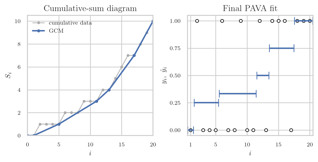
\begin{align*} \norm{\hat y- y}^2 = \ip{\hat y - y, \hat y - y} = \sum_{i=1}^n (\hat y_i - y_i)^2. \end{align*}

The greatest convex minorant method offers one way to find the isotonic fit. Form the cumulative sums \[ (0,0),\ (1,S_1),\ \ldots,\ (n,S_n), \qquad S_i = \sum_{j=1}^i y_j . \] The greatest convex minorant of these points is the largest convex function on \([0,n]\) that stays below all of them; think of a string pulled taut beneath the points, see Fig. 6.1 for an example. The isotonic fitted values \(\hat y_i\) are then the slopes of the greatest convex minorant of these cumulative points. More precisely, \(\hat y_i\) is the slope of the minorant on the segment from \(i-1\) to \(i\). We state this fact without proof; below we prove instead that PAVA solves the isotonic regression problem.

PAVA is a second method. Here we sketch its working; below we will prove that it solves the optimization problem (6.5.2).¹⁸¹⁸PAVA is supported by scikit-learn and R.

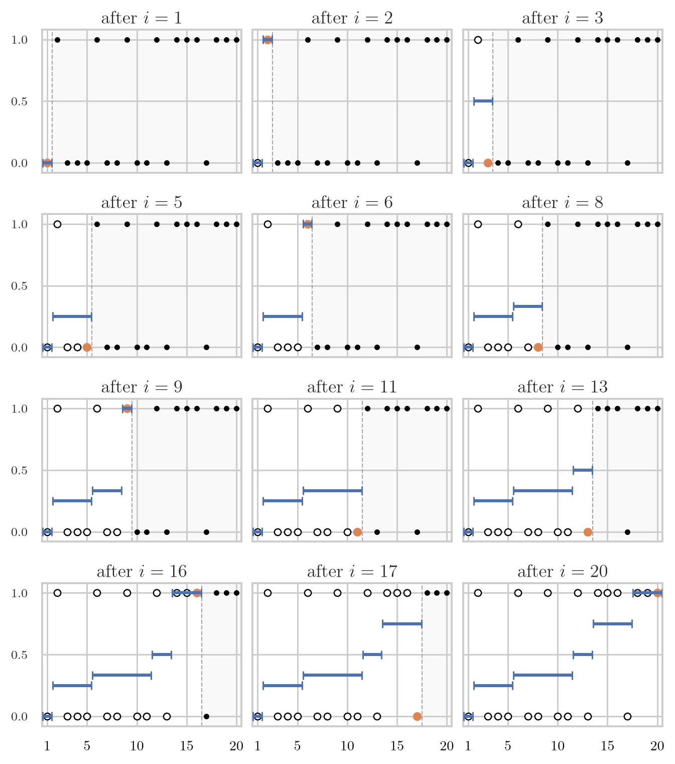
Fig. 6.2 illustrates how PAVA sweeps from left to right; Alg. 6.5.1 provides the pseudocode. It starts with one block per sorted observation, with block value \(y_i\). Whenever two neighboring blocks \(\Lset\) and \(\Rset\) violate monotonicity in that the mean label value \(\mu_\Lset\) on \(\Lset\) is larger than \(\mu_\Rset\), it merges \(\Lset\) and \(\Rset\) into a single block and replaces their values by the average of the labels \(y\) in the merged block.¹⁹¹⁹This pooled average is the barycentric mean of the two old block means, with weights given by the block sizes. In finding the greatest convex minorant this is the replacement of two adjacent violating slopes by the slope of the chord over their union. It continues merging until all block averages are nondecreasing. A careful left-to-right implementation of PAVA runs in \(O(n)\) time once the scores are sorted; the sorting step costs \(O(n\log n)\), so the full calibration procedure is typically \(O(n\log n)\).

\begin{algorithm}
\caption{Pool Adjacent Violators Algorithm}
\begin{algorithmic}
\State Start with singleton blocks $\set{1},\ldots,\set{n}$ and set $\hat y_i \gets y_i$ for all $i$.
\State Assign each block $B$ its average $\mu_B = |B|^{-1}\sum_{i\in B} y_i$.
\While{there are adjacent blocks $\Lset,\Rset$, with $\Lset$ directly left of $\Rset$, such that $\mu_\Lset>\mu_\Rset$}
  \State Merge the blocks $\Lset,\Rset$ into one block $\Lset\cup\Rset$.
  \State $\mu_{\Lset\cup\Rset}
    \gets \frac{|\Lset|\mu_\Lset+|\Rset|\mu_\Rset}{|\Lset|+|\Rset|}$.
    \Comment{Barycentric mean}
  \State $\hat y_i \gets \mu_{\Lset\cup\Rset}$ for every $i \in \Lset \cup \Rset$.
\EndWhile
\Return $\hat y$
\end{algorithmic}
\end{algorithm}

Once PAVA has produced the fitted values \(\hat y_i\), consecutive observations with the same fitted value form blocks. These blocks can be used as adaptive bins. Suppose the final blocks are \(G_m=\set{s_m,\ldots,t_m}\), \(m=1,\ldots,M\), in increasing order of the scores, where \(s_m\) and \(t_m\) are the first and the last index of block \(m\). We choose bin boundaries²⁰²⁰The PAVA fit is defined only at the observed scores in \(\Hset\); these boundaries extend it to a function on all of \([0,1]\). by setting \(c_0=0\), \(c_M=1\), and, for \(m=1,\ldots,M-1\), \[ c_m = \frac{u_{t_m}+u_{s_{m+1}}}{2}. \] With these boundaries, the bins are as in (6.4.1). Moreover, the fitted value on block \(G_m\) is its average label value, just as in (6.4.3). Hence the calibration function \(g\) is defined exactly as in (6.4.4).

Before proving that PAVA produces the isotonic fit we need some concepts from convex analysis.²¹²¹The geometric background used here is Salmon, Isotonic Regression.

We need some definitions of convexity theory first; Fig. 6.3--Fig. 6.5 illustrate these definitions. A ray is a half line emanating from the origin; in algebraic terms, if \(x\in \R^{n}\) lies in a ray, then all points \(\alpha x\) lie in the ray for \(\alpha\geq 0\).

⊕
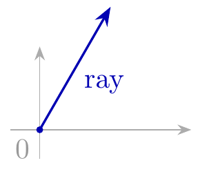
Figure 6.3: A ray starts at the origin and extends in one direction.

A cone is a set of rays, so a cone is closed under non-negative scaling. A convex set is such that when \(x\) and \(y\) lie in the set, the line segment \(\alpha x + (1-\alpha) y\), \(\alpha\in [0,1]\), between \(x\) and \(y\) lies in the set. A set is closed if its boundary belongs to it. In the sequel we will be concerned with a convex, closed and nonempty cone \(C\).

⊕
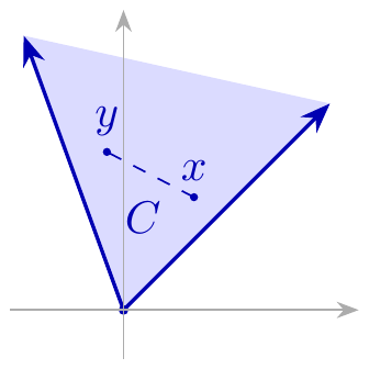
Figure 6.4: A convex cone \(C\): the segment between \(x\) and \(y\) stays in \(C\).

The last concept we need is the polar cone \(\polar{C}\) of \(C\) defined as

\begin{align*} \polar{C} = \set{z\in \R^{n} : \ip{z, x} \leq 0 \text{ for all } x \in C}. \end{align*}

The polar cone \(\polar{C}\) is also a closed convex cone. For a nonempty closed convex cone, \(\polar{\polar{C}}=C\).²²²²The word nonempty matters here. The empty set is also a closed convex cone, but every \(z\) satisfies the condition \(\ip{z, x} \leq 0\) for all \(x\in\varnothing\) vacuously, so \(\polar{\varnothing} = \R^{n}\). Consequently, \(\polar{\polar{\varnothing}} = \polar{(\R^{n})} = \set{0} \neq \varnothing\). We use this sign convention throughout; some texts reserve the term dual cone for the opposite inequality.

⊕
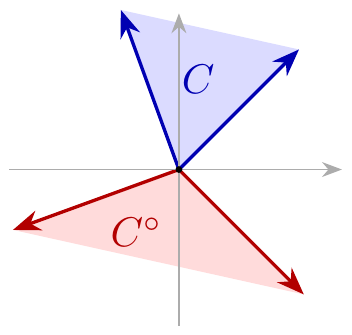
Figure 6.5: A cone \(C\) and its polar cone \(\polar{C}\).

The next two characterizations of \(\polar{C}\), in which \(A^{\top}\) denotes the transpose of the matrix \(A\) of (6.5.1), are essential to understand PAVA.

Proof

To establish the equalities, we prove the cycle of inclusions \(\polar{C}_{1} \subset \polar{C}_{2} \subset \polar{C} \subset \polar{C}_{1}\).

First we show that \(\polar{C}_{1} \subset \polar{C}_{2}\). Take \(z\in \polar{C}_{1}\) and let \(\lambda_i = \sum_{j=1}^i z_j\) as in the definition of \(\polar{C}_{1}\). With the convention \(\lambda_0 = 0\), and using that \(\lambda_n = 0\) by the definition of \(\polar{C}_{1}\), we get \(z_i=\lambda_i-\lambda_{i-1}\) for \(i=1, \ldots, n\), that is, \(z=A^{\top}\lambda\). As by assumption \(\lambda_i \geq 0\) for \(i=1,\ldots,n-1\), this shows that \(z \in \polar{C}_{2}\).

Next we prove that \(\polar{C}_{2} \subset \polar{C}\). If \(z \in \polar{C}_{2}\) then \(z=A^{\top}\lambda\) with \(\lambda\geq 0\). Consequently, \(\ip{z,x} = \ip{A^{\top}\lambda, x} = \ip{\lambda, Ax} \leq 0\) because \(Ax \leq 0\) and \(\lambda\geq 0\), hence \(z\in \polar{C}\).

Finally, we show that \(\polar{C} \subset \polar{C}_{1}\). For this we need to rewrite \(\ip{z, x}\) for \(x \in C\) in a useful way.²³²³This identity is Abel summation. It is the discrete analogue of integration by parts. Let \(\lambda_i := \sum_{j=1}^{i} z_{j}\), \(i=1, \ldots, n\), so that \(z_i = \lambda_i - \lambda_{i-1}\) if we define \(\lambda_0 = 0\). Therefore, \(\ip{z, x} = \sum_{i=1}^{n} x_i z_i = \sum_{i=1}^{n} x_i (\lambda_i - \lambda_{i-1})\). Using that \(\lambda_{0} = 0\) and relabeling,

\begin{align*} \sum_{i=1}^{n} x_{i}\lambda_{i-1} = \sum_{i=2}^{n} x_{i}\lambda_{i-1} = \sum_{i=1}^{n-1} x_{i+1}\lambda_{i}. \end{align*}

With this,

\begin{align*} \ip{z, x} = \lambda_{n} x_{n} - \sum_{i=1}^{n-1} \lambda_{i}(x_{i+1}-x_{i}). \end{align*}

This expression allows us to construct a suitable \(\lambda \in \polar{C}_{1}\) for a given \(z\in\polar{C}\). By definition of the polar cone, \(\ip{z, x}\leq 0\) for all \(x\in C\). To see that \(\lambda_n = 0\), take \(x = (1, \ldots, 1)\), which is clearly an element of \(C\). Since \(x_{i+1}-x_i=0\) in this case, \(\lambda_n x_n = \lambda_{n} \leq 0\). The constant vector \(x=(-1, \ldots, -1)\) also lies in \(C\). But then \(\ip{z, x} \leq 0\) implies that \(-\lambda_n \leq 0\). It follows that \(\lambda_n=0\). For \(\lambda_i\), \(i=1,\ldots, n-1\), take the vector \(x=(0, \ldots, 0, 1, \ldots, 1)\) with \(x_k=0\) for \(k\leq i\) and \(x_k=1\) for \(k>i\). This vector belongs to \(C\), and

\begin{align*} \ip{z, x} = \sum_{k=i+1}^n z_k = \lambda_n-\lambda_i = -\lambda_i. \end{align*}

Since \(\ip{z,x}\leq 0\), this implies that \(\lambda_i\geq 0\). Thus \(\lambda_i\geq 0\) for \(i=1,\ldots,n-1\) and \(\lambda_n=0\), so \(z\in\polar{C}_{1}\). This proves \(\polar{C}\subset\polar{C}_{1}\) and completes the proof.

We need two theorems: the projection theorem, and a decomposition theorem that builds on it.

⊕
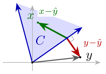
Figure 6.6: The projection theorem.

Proof

For 1, since \(C\) is nonempty, pick \(z\in C\). The intersection of \(C\) with the closed ball \(D\) with center \(y\) and radius \(\norm{z-y}\), i.e., \(D\cap C\), is compact. Since the function \(x\to\norm{x-y}\) is continuous, it attains its minimum at some point \(\hat y\) in \(D\cap C\). Any point in \(C\setminus D\) has distance greater than \(\norm{z-y}\) to \(y\), hence \(C\setminus D\) cannot contain a minimizer. Therefore \(\hat y\) minimizes the distance to \(y\) over all of \(C\).

If \(y \in C\), then \(y = P_C(y) = \hat y\): the minimal distance is \(0\), and it is attained at \(y\) only. Moreover, \(\ip{y - \hat y, x - \hat y} = 0\) for all \(x\in C\), so the inequality in 2 holds trivially. Assume therefore that \(y \notin C\), so that \(\norm{y - \hat y} > 0\).

Consider now an open ball \(B\) with center \(y\) and radius \(\norm{y-\hat y}\), hence \(\hat y \not \in B\), but \(\hat y\) is an element of the closure \(\overline B\) of \(B\). As \(\hat y\in C\) is a point closest to \(y\) in \(C\), \(B\cap C = \varnothing\). However, \(\hat y\in C\cap\overline B\), see Fig. 6.7.

Moreover, as \(C\) and \(B\) are both convex, by the separating hyperplane theorem there exists a hyperplane that separates \(B\) and \(C\). This hyperplane must pass through \(\hat y\), and as \(B\) is a ball, it is tangent to \(B\) at \(\hat y\). Consequently, the vector \(y-\hat y\) is normal to this hyperplane. As \(x\in C\) and \(y\in B\) lie at opposite sides of this plane, \(\ip{y-\hat y, x-\hat y} \leq 0\).

We can now also settle uniqueness. Any minimizer lies in \(C\cap\overline B\). Since \(C\) and \(\overline B\) lie at opposite sides of the hyperplane, \(C\cap\overline B\) is part of the hyperplane itself, and the hyperplane, being tangent to the ball, meets \(\overline B\) only at \(\hat y\). Hence \(C\cap\overline B=\set{\hat y}\): the minimizer is unique.

⊕
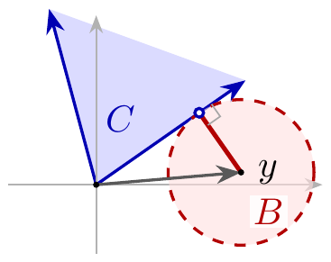
Figure 6.7: The open ball \(B\) centered at \(y\) touches the cone \(C\) at the small open circle indicating \(\hat y\). Since \(B\) is open, it is disjoint from \(C\).

Finally, suppose that \(p\in C\) is such that \(\ip{y -p, x - p} \leq 0\) for all \(x \in C\). Then

\begin{align*} \norm{y-x}^{2} = \norm{y-p + p - x}^{2} = \norm{y-p}^{2} + \norm{p-x}^{2} + 2\ip{y-p, p-x}. \end{align*}

As \(\norm{p-x} \geq 0\) and \(\ip{y-p, p-x}\ge 0\) by assumption, \(\norm{x-y} \geq \norm{y-p}\) for all \(x\in C\). Thus \(p\) is the point closest in \(C\) to \(y\), and therefore \(p=\hat y = P_C(y)\).

The projection theorem is the workhorse to prove the next theorem.

⊕
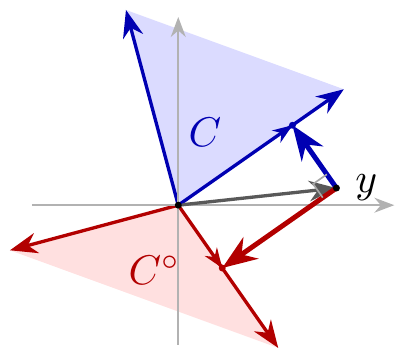
Figure 6.8: Projection arrows in Moreau’s decomposition: from \(y\) to \(\hat y=P_C(y)\) and from \(y\) to \(\polar{y}=P_{\polar{C}}(y) = y - \hat y\).

Proof

By the projection theorem, \(\hat y=P_C(y)\) exists and is unique. We first prove that \(y-\hat y \in \polar{C}\). By the projection theorem, \(\ip{y-\hat y, z - \hat y} \leq 0\) for all \(z\in C\). As \(C\) is a cone, \(0\in C\) and \(2\hat y\in C\), therefore

\begin{align*} 0 &\geq \ip{y-\hat y, 0 - \hat y} = - \ip{y - \hat y, \hat y}, \\ 0 &\geq \ip{y-\hat y, 2\hat y - \hat y} = \ip{y - \hat y, \hat y}. \end{align*}

It follows that \(\ip{y - \hat y, \hat y} = 0\). Now take any \(z\in C\). Then

\begin{align*} \ip{y - \hat y, z} &= \ip{y-\hat y, z - \hat y} + \ip{y-\hat y, \hat y}\\ &\leq 0. \end{align*}

Consequently, \(y-\hat y \in \polar{C}\).

Next we prove that \(y-\hat y=P_{\polar{C}}(y)\). Let \(p=y-\hat y\). For any \(x\in \polar{C}\),

\begin{align*} \ip{y-p, x-p} &= \ip{\hat y, x-(y-\hat y)}\\ &= \ip{\hat y, x} - \ip{\hat y, y-\hat y}\\ &\leq 0. \end{align*}

Here \(\ip{\hat y,x}\leq 0\) because \(\hat y\in C\) and \(x\in\polar{C}\), while \(\ip{\hat y,y-\hat y}=0\) by the previous paragraph. The projection theorem gives \(p=P_{\polar{C}}(y)\). Hence, with \(\polar{y}=p\),

\begin{align*} y = \hat y + \polar{y},\qquad \hat y = P_C(y),\qquad \polar{y}=P_{\polar{C}}(y),\qquad \ip{\hat y,\polar{y}}=0. \end{align*}

Finally, suppose that \(y=r+s\) with \(r\in C\), \(s\in\polar{C}\) and \(\ip{r,s}=0\). For any \(x\in C\),

\begin{align*} \ip{y-r,x-r} = \ip{s,x-r} = \ip{s,x} - \ip{s,r} \leq 0. \end{align*}

Thus \(r=P_C(y)\). Similarly, for any \(x\in\polar{C}\),

\begin{align*} \ip{y-s,x-s} = \ip{r,x-s} = \ip{r,x} - \ip{r,s} \leq 0, \end{align*}

so \(s=P_{\polar{C}}(y)\).

It remains to prove that PAVA, see Alg. 6.5.1, solves the isotonic regression problem. With the above, this reduces to showing that PAVA produces the projection \(\hat y = P_C(y)\) of the responses \(y\) on the cone \(C=\set{x\in \R^{n}: A x \leq 0}\). In other words, that it solves

\begin{align*} \hat y \in \argmin_{x: A x \leq 0} \frac{1}{2} \norm{x-y}^{2}, \end{align*}

The procedure is to focus on consecutive blocks and repair any violations of the constraint \(A x\leq 0\) one by one until no violations remain.

We also need some further notation. When \(\Iset\) is a set of consecutive indices, then we write \(y_\Iset\) for the restriction of \(y\) to \(\Iset\), and \(1_\Iset\) for the vector indexed by \(\Iset\) whose components are all \(1\). Furthermore, \(C_\Iset=\set{x \in \R^{|\Iset|} : A x \leq 0}\), where \(A\) is the matrix of (6.5.1), now of size \((|\Iset|-1)\times|\Iset|\); in words, \(C_\Iset\) consists of the nondecreasing vectors indexed by \(\Iset\).

Throughout its sweep, PAVA maintains a partition of \(\set{1,\ldots,n}\) into blocks of consecutive indices, and on each block \(\Iset = \set{a, \ldots, b}\) the current fit \(\hat y_\Iset\) is constant and equal to the block mean

\begin{align*} \mu_\Iset = \frac{1}{|\Iset|} \sum_{l \in \Iset} y_{l}. \end{align*}

The loop invariant of the algorithm is that on each block the residual \(\rscr_{\Iset,l}=y_l-\mu_\Iset\) satisfies

\begin{align*} \sum_{l=a}^{m} \rscr_{\Iset,l}\geq 0 \quad (a\leq m<b), \qquad \sum_{l=a}^{b} \rscr_{\Iset,l}=0. \end{align*}

In words, as we move through the block from left to right, the accumulated excess over the block average never becomes negative, and it is zero at the right end of the block. By the polar-cone characterization above, applied with \(n\) replaced by \(|\Iset|\), the invariant is exactly the statement that \(\rscr_\Iset\in\polar C_\Iset\). The invariant holds at the start: PAVA begins with the singleton blocks \(\set{1},\ldots,\set{n}\), so that \(\hat y = y\) and every residual is \(0\).²⁴²⁴If \(\hat y \in C\), the algorithm terminates immediately.

The invariant has an important consequence: on each block \(\Iset\), the constant vector \(\hat y_\Iset\) with components \(\mu_\Iset\) is the projection of \(y_\Iset\) on the cone \(C_\Iset\). To see this, note first that \(\hat y_\Iset\), being constant, lies in \(C_\Iset\). Second, the residual \(\rscr_\Iset = y_\Iset - \hat y_\Iset\) is orthogonal to the fit:

\begin{align*} \ip{\rscr_{\Iset}, \hat y_{\Iset}} = \ip{y_{\Iset}, \hat y_{\Iset}} -\ip{\hat y_{\Iset}, \hat y_{\Iset}} = \mu_{\Iset} \ip{y_{\Iset}, 1_{\Iset}} -\mu_{\Iset}^{2}\ip{1_{\Iset}, 1_{\Iset}} = 0, \tag{6.7.1} \end{align*}

because \(\ip{y_{\Iset}, 1_{\Iset}} = \mu_\Iset |\Iset|\) and \(\ip{1_{\Iset}, 1_{\Iset}} = |\Iset|\). Third, the invariant gives \(\rscr_\Iset\in\polar C_\Iset\). We have thus found vectors \(\hat y_\Iset \in C_\Iset\) and \(\rscr_\Iset \in \polar{C}_{\Iset}\) with \(y_\Iset = \hat y_\Iset + \rscr_\Iset\) and \(\ip{\rscr_\Iset, \hat y_\Iset} = 0\), so Moreau’s theorem shows that \(\hat y_\Iset = P_{C_\Iset}(y_\Iset)\).

Next we show that pooling two violating blocks preserves the loop invariant. Suppose that two adjacent blocks \(\Lset=\set{i,\ldots,j-1}\) and \(\Rset=\set{j,\ldots,k-1}\) violate monotonicity:

\begin{align*} \underbrace{\hat y_{i} = \cdots = \hat y_{j-1}}_{\Lset} > \underbrace{\hat y_{j} = \cdots = \hat y_{k-1}}_{\Rset}. \end{align*}

Thus \(\mu_\Lset > \mu_\Rset\). To repair this, set

\begin{align*} \mu = \frac{|\Lset| \mu_{\Lset} + |\Rset|\mu_{\Rset}}{|\Lset \cup \Rset|} = \frac{1}{|\Lset \cup \Rset|}\sum_{l\in \Lset \cup \Rset} y_l, \end{align*}

that is, the mean of the responses on the combined set \(\Lset \cup \Rset\). Observe that \(\mu_\Lset > \mu > \mu_\Rset\).

Define \(\tilde y_l = \mu\) and \(\tilde \rscr_l = y_{l} - \tilde y_l\) for \(l = i, \ldots, k-1\). Then \(\tilde y\), being constant, lies in the cone \(C_{\Lset \cup \Rset}\). To see that the pooled residual still satisfies the loop invariant, we reason as follows. On \(\Lset\), each new residual \(y_{l} - \mu\) is larger than the old residual \(y_{l} - \mu_\Lset\), so all accumulated sums inside \(\Lset\) increase; in particular, the accumulated sum at the right end of \(\Lset\) rises from \(0\) to \(|\Lset|(\mu_\Lset-\mu) > 0\). On \(\Rset\), each new residual is the old residual minus \(\mu - \mu_\Rset\), so after \(m\) elements of \(\Rset\) the accumulated sum has dropped by \(m(\mu-\mu_\Rset)\), which is at most \(|\Rset|(\mu - \mu_\Rset)\). The definition of the pooled mean gives

\begin{align*} |\Lset|(\mu_\Lset-\mu) =|\Rset|(\mu - \mu_\Rset), \end{align*}

so the drop on \(\Rset\) never exceeds the surplus gained at the right end of \(\Lset\). Since the old partial sums within \(\Rset\) are themselves nonnegative by the invariant on \(\Rset\), no accumulated sum of the merged block becomes negative. Moreover, at the right end of the merged block the surplus and the deficit cancel exactly, so the total sum is \(0\). We therefore have \(\tilde y \in C_{\Lset \cup \Rset}\) and \(\tilde \rscr \in \polar{C}_{\Lset \cup \Rset}\), and the same computation as in (6.7.1) shows that \(\ip{\tilde \rscr, \tilde y} = 0\). Thus, with Moreau’s theorem, \(\tilde y\) is the projection of the responses on the cone \(C_{\Lset \cup \Rset}\).

It is interesting to see why we should not merge when \(\mu_\Lset < \mu_\Rset\). In this case \(\mu > \mu_\Lset\), so the accumulated sum at the right end of \(\Lset\) drops from \(0\) to \(|\Lset|(\mu_\Lset - \mu) < 0\): the pooled residual violates the partial-sum condition, that is, \(\tilde \rscr \not\in \polar{C}_{\Lset \cup \Rset}\).

The last step is to establish termination and to assemble the blocks. Each pooling step reduces the number of blocks by one, and the algorithm starts with \(n\) blocks, so it terminates after at most \(n-1\) pooling steps. Upon termination no violations remain, so \(\hat y \in C\). The accumulated sums of the full residual \(\rscr = y - \hat y\) consist of sums over complete blocks, which are \(0\), plus a partial sum inside one block, which is nonnegative; in particular the total sum is \(0\). By the polar-cone characterization, \(\rscr \in \polar{C}\). Finally, \(\ip{\rscr, \hat y}\) is the sum of the block-wise inner products \(\ip{\rscr_\Iset, \hat y_\Iset}\), each of which is \(0\) by (6.7.1). Moreau’s theorem now yields \(\hat y = P_C(y)\): PAVA indeed solves the isotonic regression problem.

The KKT conditions connect the geometric projection proof to constrained optimization. The projection of \(y\) on the cone \(C\) is the constrained optimization problem

\begin{align*} \min_{x \in C} \frac{1}{2} \norm{x - y}^{2}. \end{align*}

We take this problem as the primal problem and derive its dual. This shows that the polar-cone residual in Moreau’s theorem is the dual optimizer, and that orthogonality becomes complementary slackness. The Lagrangian is

\begin{align*} \mathcal L(x, \lambda) = \frac{1}{2} \norm{x - y}^{2} + \ip{\lambda, Ax}, \quad \lambda \in \R^{n-1}_{+}. \end{align*}

Setting the derivative of \(\mathcal L\) with respect to \(x\) to \(0\) and solving for \(x\) gives \(x=y - A^{\top} \lambda\). Write this solution as \(\hat y = y - A^{\top} \lambda\). Inserting this in the Lagrangian gives the dual problem

\begin{align*} \max_{\lambda \geq 0} \set{- \frac{1}{2} \norm{A^{\top} \lambda}^{2} + \ip{\lambda, Ay}}. \end{align*}

Now define \(\rscr=A^{\top} \lambda\), so that the dual objective becomes \(-\frac{1}{2} \norm{\rscr}^{2} + \ip{\rscr, y}\) with \(\rscr\in \polar{C}\), by the second characterization of the polar cone in Lem. 6.6.1. Completing the square gives

\begin{align*} -\frac{1}{2} \norm{\rscr}^{2} + \ip{\rscr, y} = -\frac{1}{2}\norm{y-\rscr}^{2} + \frac{1}{2} \norm{y}^{2}. \end{align*}

Since the last term is a constant, maximizing the dual is the same as

\begin{align*} \min_{\rscr\in \polar{C}} \frac{1}{2}\norm{y-\rscr}^{2}. \end{align*}

This is precisely the projection of \(y\) on \(\polar{C}\). The projections of \(y\) on \(C\) and on \(\polar{C}\) solve the primal and the dual problem simultaneously.

The projection theorem gives unique solutions on \(C\) and on its polar cone \(\polar{C}\). As \(\hat y = P_C(y) \in C\), \(\hat y\) satisfies primal feasibility, likewise \(\rscr = y - \hat y \in \polar{C}\), hence \(\rscr\) satisfies dual feasibility. By Moreau’s theorem, \(0=\ip{\rscr, \hat y} = \ip{A^{\top} \lambda, \hat y} = \ip{\lambda, A\hat y}\). Since \(\lambda_i \geq 0\) and \((A\hat y)_i \leq 0\), every term of this sum is nonpositive, so each must be zero: \(\lambda_i (A\hat y)_i = 0\) for all \(i\), which is complementary slackness. And finally, \(\hat y - y + A^{\top} \lambda = 0\) is the stationarity of the Lagrangian at the optimal \(x\).

Three limits are worth stating before we move on, but let us first summarize what we did above. We began with a number the forest already produces, the fraction of its trees that vote bad, and ended with a function \(g\) that turns that number into a probability we are willing to use as a routing cost. Three methods did the turning, and they differ in just two respects: the shapes they allow for \(g\), and the loss they minimize. Sigmoid scaling allows a two-parameter S-curve and minimizes the cross-entropy that the Bernoulli likelihood selects; histogram binning allows any step function on a fixed set of bins and minimizes squared error, which the bin averages solve outright; isotonic regression allows any non-decreasing function and minimizes that same squared error under the ordering constraint, which is what PAVA computes. The fitting itself was nowhere the hard part: for sigmoid scaling it is the gradient descent of Chapter 5, and for the other two an average or a projection that we can write down.

All three methods fit \(g\) on a single held-out list \(\Hset\), and all three assume that the scores the forest produces later are distributed as the scores in \(\Hset\). This assumption is invisible in the result: a fitted \(g\) does not report that the forest beneath it has drifted, and it will keep returning confident-looking probabilities long after it has stopped deserving them. If the map, the feature set, or the training sample changes, the calibration has to be refitted, and the only protection is to refit whenever anything upstream of \(g\) changes. This is the distribution shift of Chapter 3 in calibration clothing.

Isotonic regression returns a function that is defined only at the observed scores \(u_1,\ldots,u_n\), because what the fit produces is a list of \(n\) numbers rather than a formula. Extending it to all of \([0,1]\) is a separate choice, and there is more than one reasonable one: keep \(g\) piecewise-constant and jump between blocks, or interpolate linearly between consecutive fitted values. Sigmoid scaling has no such problem, since it returns a formula that can be evaluated at any score at all, and histogram binning has none either as long as the bins cover \([0,1]\).

Scores outside the range seen in \(\Hset\) are where all three methods are weakest, and for much the same reason. There the calibrated value is an extrapolation rather than a fitted probability: sigmoid scaling evaluates its S-curve without complaint, while histogram binning and isotonic regression can do no more than repeat their outermost value. Since \(\Hset\) is held out from the training data it is typically small, so the range of scores it covers can be noticeably narrower than the range the forest produces over the whole map. This is a real concern rather than a formality: the edges with the most extreme scores are exactly the ones a router acts on most decisively.

With that said, we have assembled all the conceptual steps needed to build the app that creates walks between points \(A\) and \(B\). In Chapter B we turn to the technical details of doing so.